In the data processing work-flow for scanning mapping measurements, a wide variety and large volume of data attributes may need to be extracted and analyzed. Therefore new classes, h5xs_an and h5xs_scan, are created to provide more flexibility. A new h5 file is created for the processed data, while the raw data are kept separately in their original h5 files. The processed data are organized in a proc_data dictionary, organized in three levels:

• Sample name. This could be the sample name defined in the scan when collecting the raw data, or overall, if the final results are assembled from multiple raw data files.
  

• Data key. Here are a few already used in lixtools:

  Iqphi for the 2D intensity map as a function of scattering vector \(q\) and azimuthal angle \(\phi\);

  Iq for azimuthally averaged intensity;

  attrs for per-frame attributes extracted from the data;

  maps for structural maps reformatted from attrs based on the scan parameters;

  tomo for tomograms reconstructed from maps.
  

• Sub key. For instance, merged and subtracted for Iq, transmission and incident for attrs.

Here's an example of typical code for data processing. First we instantiate the h5xs_scan object:

from lixtools.hdf import h5xs_scan

rn = "time_series1"
dt = h5xs_scan(f"{rn}_an.h5", [de.detectors, qgrid], Nphi=61, pre_proc="2D", 
               replace_path={"legacy": "proposals"})

de defines the detectors as in solution scattering. Nphi specifies the number of azimuthal angles (evenly spaced) to be used for pre-processing that generates the \(q\)-\(\phi\) maps, as specified by pre_proc. The replace_path argument is necessary since currently the h5 files for raw data must be moved to the proposal directory manually.

Next we connect the h5xs_scan to the raw data files and import the metadata from the scans that produced the raw data:

for fn in sorted(glob.glob(f"{rn}-*.h5")):
    dt.import_raw_data(fn, force_uniform_steps=True, prec=0.001, debug=True)

Now we can perform the pre-processing, using multi-processing:

dt.process(N=8, debug=True)

Once the \(q\)-\(\phi\) maps are produced, the attributes can be generated and reorganized into maps:

for sn in dt.samples:
    dt.extract_attr(sn, "int_saxs", get_roi, "qphi", "merged", 
                    qphirange=[0.02, 0.05, -180, 180])
    dt.extract_attr(sn, "hop", hop, "qphi", "merged", xrange=[0.04, 0.06])

dt.make_map_from_attr(save_overall=False, 
                      attr_names=["transmitted", "absorption", "int_saxs", "hop"], 
                      correct_for_transsmission=False)

The extract_attr() method extracts an attribute from the processed data under sample name sn, data key qphi, and sub key merged, using the the user-specified/defined function (get_roi or hop), whose first argument must be the input data, with the specified keyword arguments (qphirange or xrange).

During and after processing, the data can be visualized using a GUI: Or the data can plotted using matplotlib: 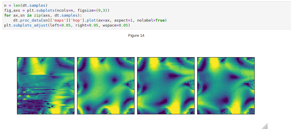In this examples, the 4 measurements('samples') correspond to 4 data points in time as a flow field is established. In some cases, these measurements could correspond to parts of a larger sample, the individual maps can then be merged based on the coordinates in the metadata from the scans.