The descriptions here are applicable for all measurements in which the scattering data is isotropic and background subtraction may be necessary. At LiX we support these measurements using two different data collection methods, typically referred to as the flow-cell measurements and the fixed cell measurements.

Flow-cell measurements

The sample is flowed from a PCR tube in the sample holder through the flow-cell, as scattering data are recorded. The instrumentation for automated measurements is described here. The samples in the holder must be specified in a spreadsheet to facilitate automated data collection and processing. Further information can be found on the LiX beamline wiki .

This method is typically used for protein samples in aqueous solution. A matching buffer must also be measured, in the same flow channel to ensure reproducible sample thickness and background scattering. Buffer scattering is subtracted based on the intensity of the water peak. It is assumed that the contribution of empty cell scattering is minimal, once the buffer scattering subtracted. For this assumption to be valid, the sample and the buffer should be measured close in time, ideally back-to-back, to avoid change in background scattering due to accumulation of materials on the flow-cell window. Also the protein concentration (volume fraction) should be reasonably low. See our workbench presentations for a more detailed discussion.

After data collection is completed for each sample holder, data from all samples are packed into a h5 file. As automated data processing takes place, the processed data are added to the same h5 file. And a html data processing report is produced. The process typically consists of the following steps:

Define the python object that corresponds to the dataset

from lixtools.hdf import h5sol_HT
from lixtools.samples import get_sample_dicts

dt = h5sol_HT(h5_file_name, (de.detectors, de.grid))

Here the class h5sol_HT is specific to the flow-cell measurements. de should be an instance of DetectorConfig (see docs for py4xs). Utilities under py4xs and reference data provided by the beamline should be used to verify the validity of de.

Assign the sample-buffer relationship and process the data

sd = get_sample_dicts(spreadSheet, holderName, use_flow-cell=True)
dt.assign_buffer(sd['buffer'])
dt.process(sc_factor='auto', debug='quiet')

The last line performs azimuthal averaging, frame selection, and buffer subtraction. These can be done separately. Refer to the code under lixtools.

Generate processing report

from lixtools.atsas import gen_report

gen_report(h5_file_name)

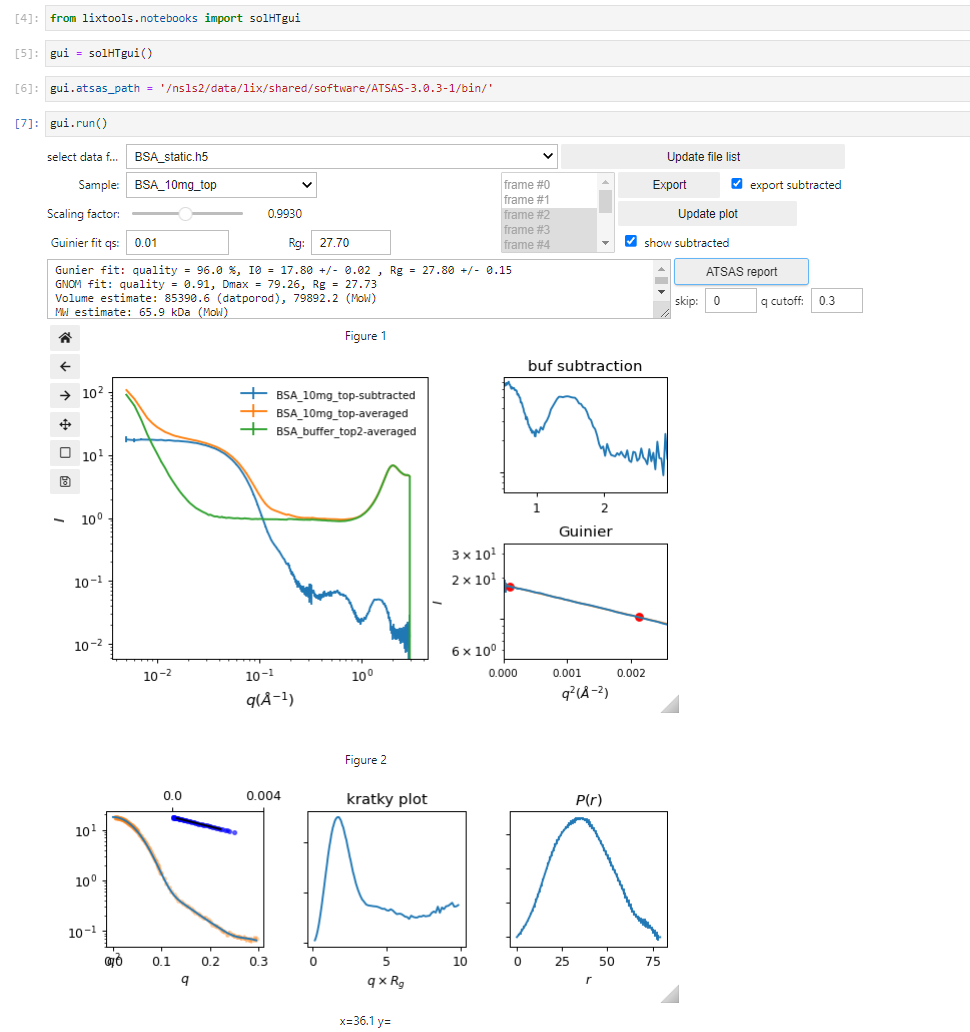
This will produce a html report for all samples in the h5 file. Things could go wrong during automated data processing. The processing report provides an overview of the processing results and provide a guide on whether frame selection for averaging and scaling for buffer subtraction need to be adjusted. These adjustment can be done by using the data visualization GUI or by code.

Fixed cell measurements

Alternatively, the sample can be scanned such that the x-ray beam moves across the sample as scattering data are collected. The sample will need to be pre-loaded into a multi-position sample holder. We support multiple holder formats. Again, consult the beamline wiki regarding the sample holders and the required spreadsheet for automated data processing. With fixed cell measurements it is important to specify how empty cell scattering should be subtracted.

The data processing work-flow is slightly different from flow-cell measurements:

from lixtools.hdf import h5sol_fc
from lixtools.samples import get_sample_dicts

dt = h5sol_fc(f'{sample_hn}.h5', [de.detectors, de.qgrid])

sd = get_sample_dicts(spreadSheet, holderName)
dt.assign_empty(sd['empty'])
dt.assign_buffer(sd['buffer'])

dt.process(rebin_data=True, trigger="ss_y", sc_factor='auto')

A few important differences: (a) the h5sol_fc class should be used; (b) both buffer and empty cell need to be specified; (c) the motor used to scan the sample should be specified. Again, a GUI is provided for tweaking the processing parameters and data visualization.

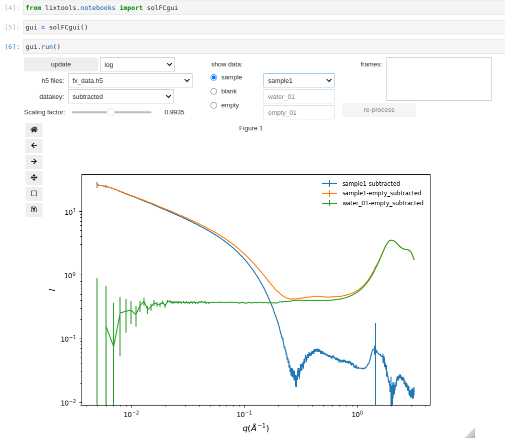
The ATSAS report is not provided since the data often contain the contribution from a structure factor due to interactions between the particles in solution, or the structure cannot be considered as particles. Instead, the data can be exported into a NXcanSAS file for analysis in sasview:

gui.dt.export_NXcanSAS()

Common utilities

Both h5sol_HT and h5sol_HT are derived from the h5xs class from py4xs, and therefore can access methods described under h5xs docs. For instance, once the data processing is done once, the 1D data can be reloaded from the h5 file using load_d1s(), visualized using plot_d1s(), compared between different samples in the same file using compare_d1s(), and exported using export_d1s().

Frame selection

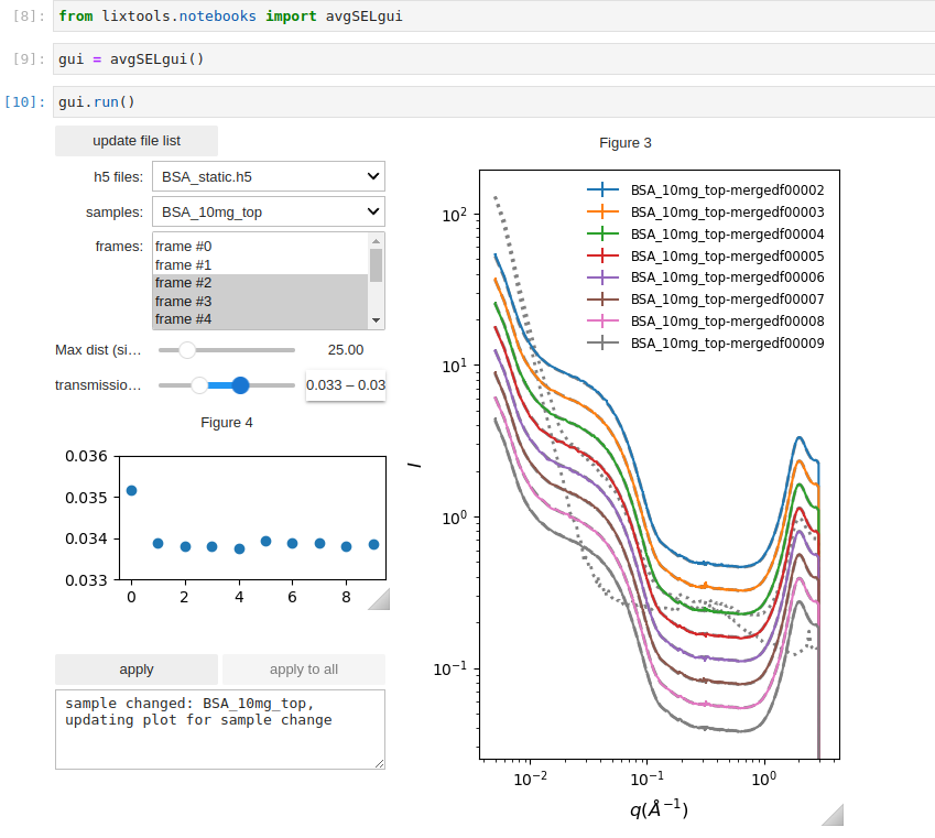
In some situations, the scattering patterns (typically 10-20 frames) collected from the same sample may be different. This can happen if bubbles form when the sample is loaded into the flow cell, or if there is not enough sample to cover the entire scan range in the fixed cell. It is therefore necessary to exclude the frames that do not correspond to the beam fully illuminating the sample. While simple similarity comparison is often sufficient, it is more reliable to also check the x-ray transmission through the sample, which is expected to be higher is the beam-illuminated volume is not completely filled with sample. This GUI below is useful for identifying what the threshold values should be for transmission and similarity (max pairwise distance), so that they can be applied in automated frame selection.

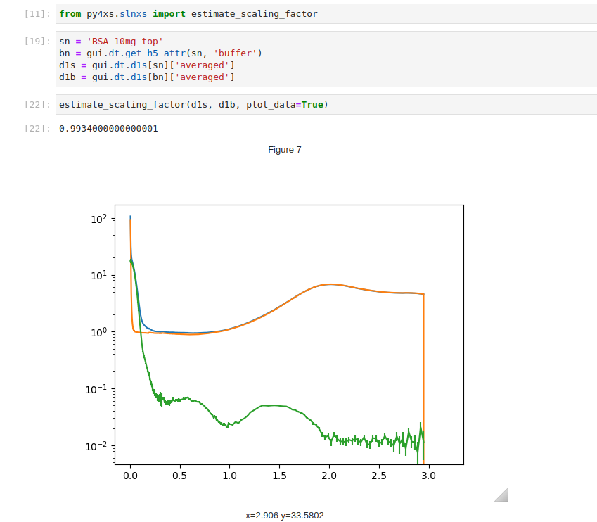
Scaling factor estimate

As discussed here, subtraction of the scattering from the aqueous buffer can be performed based on the intensity of the water peak, which automatically takes into account the volume fraction occupied by the solute molecules. However, an additional scaling factor is still necessary and need to be fine tuned. This scaling factor can be estimated using the estimate_scaling_factor() function.

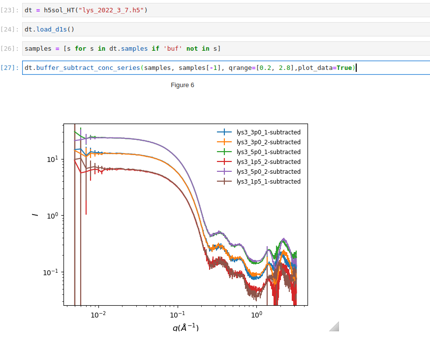
For a concentration series, the scaling factor can be adjusted in coordination, assuming that the shape of the high-\(q\) data should be independent of the concentration after the subtraction .